Burgers 방정식#
강좌: 기초 전산유체역학
%matplotlib inline
from matplotlib import pyplot as plt

import numpy as np

plt.style.use('ggplot')
plt.rcParams['figure.dpi'] = 150
Burgers 방정식#
Burgers 방정식은 다음과 같이 표현된다.
비 보존형의 경우 다음과 같이 표현할 수 있다.
이 방정식은 운동량 보존식에서 비선형 항만 표현한 식이다.
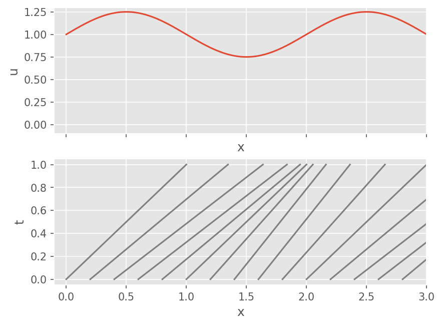
선형 파동 방정식과 비교했을 때, 각 지점에서 교란의 전파 속도는 \(u\) 이다. 즉 \(x-t\) 그래프에서 Characteristic의 기울기가 해 \(u\) 에 따라 달라진다.
x = np.linspace(0, 3, 151)
u = 1+ 0.25*np.sin(np.pi*x)
t = np.linspace(0, 1, 101)

fig, axs = plt.subplots(2, 1, sharex=True)
axs[0].plot(x, u)
axs[0].set_xlim(-0.1, 3)
axs[0].set_ylabel('u')
axs[0].set_ylim(-0.1, 1.3)
axs[0].set_xlabel('x')

for i in range(15):
    xi, ui = x[10*i], u[10*i]

    # Characteristics with the wave speed u
    xx = xi + ui*t
    axs[1].plot(xx,t, color='gray')

axs[1].set_ylabel('t')
axs[1].set_xlabel('x')
Text(0.5, 0, 'x')
Riemann Problem의 해#
다음 Riemann Problem를 생각하자.
2가지 해가 존재한다.
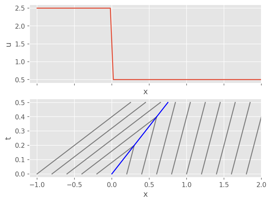
Shock#
\(u_L > u_R\) 인 경우 불연속 충격파가 발생한다. 충격파의 속도는 Rankine-Hugoniot Jump 조건을 통해 구할 수 있다.
x = np.linspace(-1, 2, 151)
u = -np.tanh(1e8*x) + 1.5
t = np.linspace(0, 0.5, 101)

fig, axs = plt.subplots(2, 1, sharex=True)
axs[0].plot(x, u)
axs[0].set_xlim(-1.1, 2)
axs[0].set_ylabel('u')
axs[0].set_xlabel('x')

xs = 1.5*t

for i in range(15):
    xi, ui = x[10*i], u[10*i]

    # Characteristics with the wave speed u
    xx = xi + ui*t

    # Do not draw characteristics after shcok
    idx1 = np.argmin(xx < xs)
    idx2 = np.argmax(xx < xs)

    if idx1 + idx2 == 0:
        if xi != 0:
            axs[1].plot(xx, t, color='gray')
    else:
        if idx1 > 0:
            axs[1].plot(xx[:idx1], t[:idx1], color='gray')
        else:
            axs[1].plot(xx[:idx2], t[:idx2], color='gray')

# Rankine Hugoniot condtion
axs[1].plot(xs, t, color='blue')

axs[1].set_ylabel('t')
axs[1].set_xlabel('x')
Text(0.5, 0, 'x')
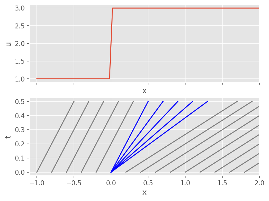
Rarefaction#
\(u_L < u_R\) 인 경우 해는 연속적으로 팽창한다. 이 때 해는 \(x/t\) 에 Self-similar 하다. 현재 시간과 경계에 대한 국소 좌표계를 \(\hat{t}\), \(\hat{x}\) 에 대해서 Self-similar 한 해 \(\hat{u}\)는 다음과 같다.
x = np.linspace(-1, 2, 151)
u = np.tanh(1e8*x) + 2
t = np.linspace(0, 0.5, 101)

fig, axs = plt.subplots(2, 1, sharex=True)
axs[0].plot(x, u)
axs[0].set_xlim(-1.1, 2)
axs[0].set_ylabel('u')
axs[0].set_xlabel('x')

for i in range(15):
    xi, ui = x[10*i], u[10*i]

    # Characteristics with the wave speed u
    xx = xi + ui*t

    if xi != 0:
        axs[1].plot(xx, t, color='gray')

# Expansion fan
for i in range(5):
    axs[1].plot((1+2/5*i)*t, t, color='blue')

axs[1].set_ylabel('t')
axs[1].set_xlabel('x')
Text(0.5, 0, 'x')
Entropy Condition#
쌍곡 보존식의 해는 팽창파 뿐 아니라 팽창충격파도 존재할 수 있다. 그러나 자연 현상에서는 점성에 의해 팽창파만 존재한다. 즉 엔트로피가 증가하는 방향으로만 해가 존재한다.
Burgers 방정식에서도 Entropy 조건을 만족해야 한다.
볼연속 충격파의 전파 속도는 다음 조건을 만족한다.
수치해석#
앞선 선형 방정식과 같이 다음 Finite Volume Method 식으로 계산한다.
\[ U_i^{n+1} = U_i^n - \frac{\Delta t}{\Delta x} \left ( F^n_{i+1/2} - F^n_{i-1/2} \right ) \]\(F^n_{i+1/2} = \frac{1}{\Delta t} \int_{t^n}^{t^{n+1}} f(u(x_{i+1/2}, t) dt\)
\(F^n_{i+1/2} \approx \mathcal{F} (U_i^n, U_{i+1}^n)\)
Flux를 제외한 수치 방법은 동일하다.
시간 간격 계산시 Wave speed \(f'(u)=u\)가 위치별로 다르므로, 최대값을 사용한다.
Runge Kutta 등의 다양한 시간 적분 기법을 적용하기 위해 다음과 같이 Semi-discrete form으로 계산할 수 있다.
\[ \frac{dU_i}{dt} = - \frac{1}{\Delta x} (F_{i+1/2} - F_{i-1/2}) \]
Godunov Method#
Exact Riemann Prolbem을 해석해서 계산한다.
\(F^n_{i+1/2} \approx f(u^n_{i+1/2})\)
\(u^n_{i+1/2}\) 는 Exact Riemann Problem으로 Shock wave 와 Expansion Wave 결과로 계산한다.
Approximate Riemann solver#
간단한 Burgers 방정식의 경우 Exact Riemann Problem 계산이 가능하나, Euler 등의 System 방정식에서 Riemann Problem을 해석하는 것은 어렵다.
수치 안정적인 Upwind 기법 적용이 가능하다.
\[ F^n_{i+1/2} = \mathcal{F} (U_i^n, U_{i+1}^n) = \frac{1}{2} \left [ f(U_i^n) + f(U_{i+1}^n) \right ] - \frac{1}{2} |a_{i+1/2}| \left ( U_{i+1}^n - U_i^n \right ) \]여기서 Intercell에서 Wavespeed는 \(|a_{i+1/2}|=S\) 로 한다.
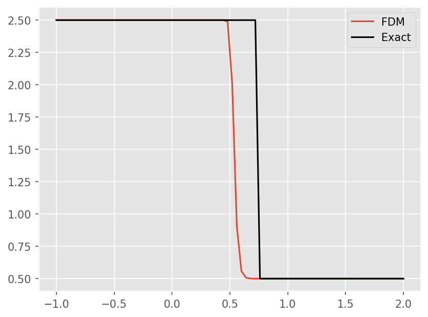
Converavtive vs Non-conservative#
Finite Volume method for conservative form
Finite Difference method for non-conservative form
(Lax and Wendroff) 수치해가 수렴하기 위해서는 weak form 을 만족해야 한다. 즉 jump condition을 만족해야 한다.
# Finite Difference Method
t_target = 0.5
cfl = 0.9

# Make grid
nx = 75
x = np.linspace(-1, 2, nx+1)
dx = np.diff(x)[0]

# Solution array
u = np.empty(nx+3)
du = np.zeros_like(u)

# Upwind scheme
def upwind(nx, u, du, dt, dx):
    for i in range(1, nx+2):
        du[i] = -u[i] * (u[i] - u[i-1])*dt/dx

# Transparent BC
def bc_transparent(u):
    u[0] = u[1]
    u[-1] = u[-2]

# Initialize
u[1:-1] =  -np.tanh(1e8*x) + 1.5
bc_transparent(u)

# Calculation
t = 0
while abs(t - t_target) > 1e-8:
    # Adjust time step to reach target time
    dt = cfl*dx / abs(u[1:-1]).max()
    dt = min(dt, t_target - t)

    # Periodic BC
    bc_transparent(u)

    # Non-conservative Upwind
    upwind(nx, u, du, dt, dx)

    # Update
    u += du
    t += dt

# Plot solution
plt.plot(x, u[1:-1])

# Plot exact
s = 0.5*(u[0] + u[-1])
plt.plot(x, -np.tanh(1e8*(x - s*t)) + 1.5, color='k')

plt.legend(['FDM', 'Exact'])
<matplotlib.legend.Legend at 0x7f0a147d9010>
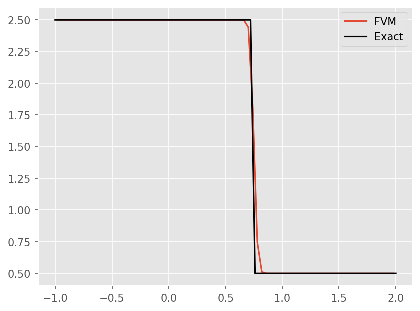
# Finite Volume Method
t_target = 0.5
cfl = 0.9

# Make grid
nx = 75
x = np.linspace(-1, 2, nx+1)
dx = np.diff(x)[0]
xc = x[:-1] + 0.5*dx

# Solution and flux array
u = np.empty(nx+2)
f = np.empty(nx+1)

# Upwind flux
eps = 1e-10

def upwind(nx, u, f):
    for j in range(nx+1):
        ul, ur = u[j], u[j+1]

        fl = 0.5*ul**2
        fr = 0.5*ur**2

        s = (fr - fl + eps) / (ur - ul + eps)

        f[j] = (fl + fr)/2 - abs(s)/2*(ur - ul)

# Initialize
u[1:-1] =  -np.tanh(1e8*xc) + 1.5

# Calculation
t = 0
while abs(t - t_target) > 1e-8:
    # Adjust time step to reach target time
    dt = cfl*dx / abs(u[1:-1]).max()
    dt = min(dt, t_target - t)

    # Periodic BC
    bc_transparent(u)

    # Compute Flux
    upwind(nx, u, f)

    # Update solution and time
    u[1:-1] -= dt/dx * (f[1:] - f[:-1])
    t += dt

# Plot solution
plt.plot(xc, u[1:-1])

# Plot exact
s = 0.5*(u[0] + u[-1])
plt.plot(x, -np.tanh(1e8*(x - s*t)) + 1.5, color='k')

plt.legend(['FVM', 'Exact'])
<matplotlib.legend.Legend at 0x7f0a147c2cd0>
예제#
Burgers 방정식을 생각하자.
계산 영역은 \([-1,1]\) 이다. 아래 유동을 유한체적법으로 계산하시오. Flux 기법은 Upwind를 사용하시오.
아래 초기 조건에 대해서 Tranparent 경계 조건이고 \(t=0.5\) 일 때 계산하시오. Rankine-Hugoniot 조건을 이용해서 충격파의 Wave speed를 예측하는지 확인하시오.
\[\begin{split} u(x,0) = \left \{ \begin{array}{cc} 1.5 & x \le 0 \\ 0.5 & else \end{array} \right. \end{split}\]아래 초기 조건에 대해서 Tranparent 경계 조건이고 \(t=0.5\) 일 때 계산하시오. Entropy 조건을 만족하는지 확인하시오.
\[\begin{split} u(x,0) = \left \{ \begin{array}{cc} 0.5 & x \le 0 \\ 1.5 & else \end{array} \right. \end{split}\]초기 조건이 \(u(x,0) = 1 + 0.5 \sin(\pi x)\) Periodic 경계조건 인 경우 \(t=0.5, 1.0, 1.5\) 일 때 계산하시오. \(x-t\) 그래프를 그려보고 수치해와 이론해를 비교 분석하시오.
다음과 같이 조건을 변경하면서 계산하시오.
CFL 수를 바꿔가면서 계산하시오.
격자 개수 (\(nx=50, 100, 200, 400\))를 다르게 하면서 변화를 확인하시오.